A tour through HTSeq

This tour demonstrates the functionality of HTSeq by performing a number of common analysis tasks:

• Getting statistical summaries about the base-call quality scores to study the data quality.
• Calculating a coverage vector and exporting it for visualization in a genome browser.
• Reading in annotation data from a GFF file.
• Assigning aligned reads from an RNA-Seq experiments to exons and genes.

The following description assumes that the reader is familiar with Python and with HTS data. (For a good and not too lengthy introduction to Python, read the Python Tutorial on the Python web site.)

If you want to try out the examples on your own system, you can download the used example files here: HTSeq_example_data.tgz

Reading in reads

In the example data, a FASTQ file is provided with example reads from a yeast RNA-Seq experiment. The file yeast_RNASeq_excerpt_sequence.txt is an excerpt of the _sequence.txt file produced by the SolexaPipeline software. We can access it from HTSeq with

>>> import HTSeq
>>> fastq_file = HTSeq.FastqReader( "yeast_RNASeq_excerpt_sequence.txt", "solexa" )

The first argument is the file name, the optional second argument indicates that the quality values are encoded according to Solexa’s specification. If you omit it, the default “phred” is assumed, which means the encoding originally suggested by the Sanger Institute. (A third option is “solexa_old”, for data from the SolexaPipeline prior to version 1.3.)

The variable fastq_file is now an object of class FastqReader, which refers to the file:

>>> fastq_file
<FastqReader object, connected to file name 'yeast_RNASeq_excerpt_sequence.txt'>

When used in a for loop, it generates an iterator of objects representing the reads. Here, we use the islice function from itertools to cut after 10 reads.

>>> import itertools
>>> for read in itertools.islice( fastq_file, 10 ):
...    print read
CTTACGTTTTCTGTATCAATACTCGATTTATCATCT
AATTGGTTTCCCCGCCGAGACCGTACACTACCAGCC
TTTGGACTTGATTGTTGACGCTATCAAGGCTGCTGG
ATCTCATATACAATGTCTATCCCAGAAACTCAAAAA
AAAGTTCGAATTAGGCCGTCAACCAGCCAACACCAA
GGAGCAAATTGCCAACAAGGAAAGGCAATATAACGA
AGACAAGCTGCTGCTTCTGTTGTTCCATCTGCTTCC
AAGAGGTTTGAGATCTTTGACCACCGTCTGGGCTGA
GTCATCACTATCAGAGAAGGTAGAACATTGGAAGAT
ACTTTTAAAGATTGGCCAAGAATTGGGGATTGAAGA

Of course, there is more to a read than its sequence. The variable read still contains the tenth read, and we may examine it:

>>> read
<SequenceWithQualities object 'HWI-EAS225:1:10:1284:142#0/1'>

A Sequence object has two slots, called seq and name. This here is a SequenceWithQualities, and it also has a slot qual:

>>> read.name
'HWI-EAS225:1:10:1284:142#0/1'
>>> read.seq
'ACTTTTAAAGATTGGCCAAGAATTGGGGATTGAAGA'
>>> read.qual
array([33, 33, 33, 33, 33, 33, 29, 27, 29, 32, 29, 30, 30, 21, 22, 25, 25,
       25, 23, 28, 24, 24, 29, 29, 29, 25, 28, 24, 24, 26, 25, 25, 24, 24,
       24, 24])

The values in the quality array are, for each base in the sequence, the Phred score for the correctness of the base.

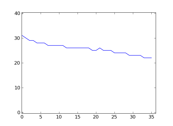
As a first simple example for the use of HTSeq, we now calculate the average quality score for each position in the reads by adding up the qual arrays from all reads and the dividing by the number of reads. We sum everything up in the variable qualsum, a numpy array of integers:

>>> import numpy
>>> len( read )
36
>>> qualsum = numpy.zeros( len(read), numpy.int )

Then we loop through the fastq file, adding up the quality scores and counting the reads:

>>> nreads = 0
>>> for read in fastq_file:
...    qualsum += read.qual
...    nreads += 1

The average qualities are hence:

>>> qualsum / float(nreads)
array([ 31.56838274,  30.08288332,  29.4375375 ,  29.00432017,
        28.55290212,  28.26825073,  28.46681867,  27.59082363,
        27.34097364,  27.57330293,  27.11784471,  27.19432777,
        26.84023361,  26.76267051,  26.44885795,  26.79135165,
        26.42901716,  26.49849994,  26.13604544,  25.95823833,
        25.54922197,  26.20460818,  25.42333693,  25.72298892,
        25.04164167,  24.75151006,  24.48561942,  24.27061082,
        24.10720429,  23.68026721,  23.52034081,  23.49437978,
        23.11076443,  22.5576223 ,  22.43549742,  22.62354494])

If you have matplotlib installed, you can plot this.

>>> from matplotlib import pyplot
>>> pyplot.plot( qualsum / nreads )    
[<matplotlib.lines.Line2D object at 0x...>]
>>> pyplot.show()                      

This is a very simple way of looking at the quality scores. For more sophisticated quality-control techniques, see the Chapter Quality Assessment with htseq-qa.

What if you did not get the _sequence.txt file from your core facility but instead the export.txt file? While the former contains only the reads and their quality, the latter also contains the alignment of the reads to a reference as found by Eland. To read it, simply use

>>> alignment_file = HTSeq.SolexaExportReader( "yeast_RNASeq_excerpt_export.txt" )  

HTSeq can also use other alignment formats, e.g., SAM:

>>> alignment_file = HTSeq.SAM_Reader( "yeast_RNASeq_excerpt.sam" )

If we are only interested in the qualities, we can rewrite the commands from above to use the alignment_file:

>>> nreads = 0
>>> for aln in alignment_file:
...    qualsum += aln.read.qual
...    nreads += 1

We have simple replaced the FastqReader with a SolexaExportReader, which iterates, when used in a for loop, over SolexaExportAlignment objects. Each of these contain a field read that contains the SequenceWithQualities object, as before. There are more parses, for example the SAM_Reader that can read SAM files, and generates SAM_Alignment objects. As all Alignment objects contain a read slot with the SequenceWithQualities, we can use the same code with any alignment file for which a parser has been provided, and all we have to change is the name of the reader class in the first line.

The other fields that all Alignment objects contain, is a Boolean called aligned that tells us whether the read has been aligned at all, and a field called iv (for “interval”) that shows where the read was aligned to. We use this information in the next section.

Genomic intervals and genomic arrays

Genomic intervals

At the end of the previous section, we looped through a SAM file. In the for loop, the SAM_Reader object yields for each alignment line in the SAM file an object of class SAM_Alignment. Let’s have closer look at such an object, still found in the variable aln:

>>> aln
<SAM_Alignment object: Read 'HWI-EAS225:1:11:76:63#0/1' aligned to IV:[246048,246084)/+>

Every alignment object has a slot read, that contains a SequenceWithQualities object as described above

>>> aln.read
<SequenceWithQualities object 'HWI-EAS225:1:11:76:63#0/1'>
>>> aln.read.name
'HWI-EAS225:1:11:76:63#0/1'
>>> aln.read.seq
'ACTGTAAATACTTTTCAGAAGAGATTTGTAGAATCC'
>>> aln.read.qual
array([33, 33, 33, 33, 31, 33, 30, 32, 33, 30, 29, 33, 32, 32, 32, 31, 32,
       31, 29, 28, 30, 28, 30, 24, 28, 30, 28, 26, 24, 29, 24, 23, 23, 27,
       25, 25])

Furthermore, every alignment object has a slot iv (for “interval”) that describes where the read was aligned to (if it was aligned). To hold this information, an object of class GenomicInterval is used that has slots as follows:

>>> aln.iv
<GenomicInterval object 'IV', [246048,246084), strand '+'>
>>> aln.iv.chrom
'IV'
>>> aln.iv.start
246048
>>> aln.iv.end
246084
>>> aln.iv.strand
'+'

Note that all coordinates in HTSeq are zero-based (following Python convention), i.e. the first base of a chromosome has index 0. Also, all intervals are half-open, i.e., the end position is not included. The strand can be one of '+', '-', and '.', where the latter indicates that the strand is not defined or not of interest.

Apart from these slots, a GenomicInterval object has a number of convenience functions, see the reference.

Note that a SAM file may contain reads that could not be aligned. For these, the iv slot contains None. To test whether an alignment is present, you can also query the slot aligned, which is a Boolean.

Genomic Arrays

The GenomicArray data structure is a convenient way to store and retrieve information associated with a genomic position or genomic interval. In a GenomicArray, data (either simple scalar data like a number) or can be stored at a place identified by a GenomicInterval. We demonstrate with a toy example.

Assume you have a genome with three chromosomes with the following lengths (in bp):

>>> chromlens = { 'chr1': 3000, 'chr2': 2000, 'chr1': 1000 }

We wish to store integer data (typecode “i”)

>>> ga = HTSeq.GenomicArray( chromlens, stranded=False, typecode="i" )

Now, we can assign the value 5 to an interval:

>>> iv = HTSeq.GenomicInterval( "chr1", 100, 120, "." )
>>> ga[iv] = 5

We may want to add the value 3 to an interval overlapping with the previous one:

>>> iv = HTSeq.GenomicInterval( "chr1", 110, 135, "." )
>>> ga[iv] += 3

To see the effect of this, we read out an interval encompassing the region that we changed. To display the data, we convert to a list:

>>> iv = HTSeq.GenomicInterval( "chr1", 90, 140, "." )
>>> list( ga[iv] )  
[0, 0, 0, 0, 0, 0, 0, 0, 0, 0, 5, 5, 5, 5, 5, 5, 5, 5, 5, 5, 8, 8, 8,
 8, 8, 8, 8, 8, 8, 8, 3, 3, 3, 3, 3, 3, 3, 3, 3, 3, 3, 3, 3, 3, 3, 0,
 0, 0, 0, 0]

It would be wasteful to store all these repeats of the same value as it is displayed here. Hence, GenomicArray objects use by default so-called StepVectors that store the data internally in “steps” of constant value. Often, reading out the data that way is useful, too:

>>> for iv2, value in ga[iv].steps():
...    print iv2, value
...
chr1:[90,100)/. 0
chr1:[100,110)/. 5
chr1:[110,120)/. 8
chr1:[120,135)/. 3
chr1:[135,140)/. 0

If the steps become very small, storing them instead of just the unrolled data may become inefficient. In this case, GenomicArrays should be instantiated with storage mode ndarray to get a normal numpy array as backend, or with storage mode memmap to use a file/memory-mapped numpy array (see reference for details).

In the following section, we demonstrate how a GenomicArray can be used to calculate a coverage vector. In the section after that, we see how a GenomicArray with type code ‘O’ (which stands for ‘object’, i.e., any kind of data, not just numbers) is useful to organize metadata.

Calculating coverage vectors

By a “coverage vector”, we mean a vector (one-dimensional array) of the length of a chromosome, where each element counts how many reads cover the corresponding base pair in their alignment. A GenomicArray can conveniently bundle the coverage vectors for all the chromosomes in a genome.

Hence, we start by defining a GenomicArray:

>>> cvg = HTSeq.GenomicArray( "auto", stranded=True, typecode='i' )

Instead of listing all chromosomes, we instruct the GenomicArray to add chromosome vectors as needed, by specifiyng "auto". As we set stranded=True, there are now two chromosome vectors for each chromosome, all holding integer values (typecode='i'). They all have an “infinte” length as we did not specify the actual lengths of the chromosomes.

To build the coverage vectors, we now simply iterate through all the reads and add the value 1 at the interval to which each read was aligned to:

>>> alignment_file = HTSeq.SAM_Reader( "yeast_RNASeq_excerpt.sam" )
>>> cvg = HTSeq.GenomicArray( "auto", stranded=True, typecode='i' )
>>> for alngt in alignment_file:
...    if alngt.aligned:
...       cvg[ alngt.iv ] += 1

We can plot an excerpt of this with:

>>> pyplot.plot( list( cvg[ HTSeq.GenomicInterval( "III", 200000, 500000, "+" ) ] ) )     
[<matplotlib.lines.Line2D object at 0x...>]

However, a proper genome browser gives a better impression of the data. The following commands write two BedGraph (Wiggle) files, one for the plus and one for the minus strands:

>>> cvg.write_bedgraph_file( "plus.wig", "+" )
>>> cvg.write_bedgraph_file( "minus.wig", "-" )

These two files can then be viewed in a genome browser (e.g. IGB), alongside the annotation from a GFF file (see below).

Counting reads by genes

As the example data is from an RNA-Seq experiment, we want to know how many reads fall into the exonic regions of each gene. For this purpose we first need to read in information about the positions of the exons. A convenient source of such information are the GTF files from Ensembl (to be found here).

These file are in the GTF format, a tightening of the GFF format. HTSeq offers the GFF_Reader class to read in a GFF file:

>>> gtf_file = HTSeq.GFF_Reader( "Saccharomyces_cerevisiae.SGD1.01.56.gtf.gz" )
>>> for feature in itertools.islice( gtf_file, 10 ):
...    print feature
...
<GenomicFeature: exon 'R0010W' at 2-micron: 251 -> 1523 (strand '+')>
<GenomicFeature: CDS 'R0010W' at 2-micron: 251 -> 1520 (strand '+')>
<GenomicFeature: start_codon 'R0010W' at 2-micron: 251 -> 254 (strand '+')>
<GenomicFeature: stop_codon 'R0010W' at 2-micron: 1520 -> 1523 (strand '+')>
<GenomicFeature: exon 'R0020C' at 2-micron: 3007 -> 1885 (strand '-')>
<GenomicFeature: CDS 'R0020C' at 2-micron: 3007 -> 1888 (strand '-')>
<GenomicFeature: start_codon 'R0020C' at 2-micron: 3007 -> 3004 (strand '-')>
<GenomicFeature: stop_codon 'R0020C' at 2-micron: 1888 -> 1885 (strand '-')>
<GenomicFeature: exon 'R0030W' at 2-micron: 3270 -> 3816 (strand '+')>
<GenomicFeature: CDS 'R0030W' at 2-micron: 3270 -> 3813 (strand '+')>

The feature variable is filled with objects of class GenomicFeature. As with all Python objects, the dir function shows us its slots and functions:

>>> dir( feature )   
['__class__', ..., '__weakref__', 'attr', 'frame', 'get_gff_line',
'iv', 'name', 'score', 'source', 'type']

Ignoring the attributes starting with an underscore, we can see now how to access the information stored in the GFF file. The information from the columns of the GFF table is accessible as follows:

>>> feature.iv
<GenomicInterval object '2-micron', [3270,3813), strand '+'>
>>> feature.source
'protein_coding'
>>> feature.type
'CDS'
>>> feature.score
'.'

The last column (the attributes) is parsed and presented as a dict:

>>> feature.attr    
{'exon_number': '1', 'gene_id': 'R0030W', 'transcript_name': 'RAF1',
'transcript_id': 'R0030W', 'protein_id': 'R0030W', 'gene_name': 'RAF1'}

The very first attribute in this column is usually some kind of ID, hence it is stored in the slot name:

>>> feature.name
'R0030W'

To deal with this data, we will use a GenomicArray. A GenomicArray can store not only numerical data but also arbitrary Python objects (with typecode ‘O’). Hence, we can assign those features that correspond to exons, to steps in the GenomicArray:

>>> exons = HTSeq.GenomicArray( "auto", stranded=False, typecode='O' )
>>> for feature in gtf_file:
...    if feature.type == "exon":
...       exons[ feature.iv ] = feature

Now, we can ask what exons occur in a certain interval:

>>> iv = HTSeq.GenomicInterval( "II", 120000, 125000, "." )
>>> list( exons[iv].steps() ) 
[(<GenomicInterval object 'II', [120000,121877), strand '.'>,
     <GenomicFeature: exon 'YBL052C' at II: 121876 -> 119380 (strand '-')>),
 (<GenomicInterval object 'II', [121877,122755), strand '.'>,
     None),
 (<GenomicInterval object 'II', [122755,124762), strand '.'>,
     <GenomicFeature: exon 'YBL051C' at II: 124761 -> 122754 (strand '-')>),
 (<GenomicInterval object 'II', [124762,125000), strand '.'>,
     None)]

However, our RNA-Seq experiment was not strand-specific, i.e., we do not know whether the reads came from the plus or the minus strand. This is why we defined the GenomicArray as non-stranded (stranded=False in the instantiation of exons above), instructing it to ignore all strand information. An issue with this is that we now have many overlapping genes and the simple assignment exons[ feature.iv ] = feature is overwriting, so that it is not clear which feature we set.

The proper solution is to store not just single features at an interval but sets of all features which are present there. A specialization of GenomicArray, GenomicArrayOfSets is offered to simplify this:

>>> exons = HTSeq.GenomicArrayOfSets( "auto", stranded=False )

We populate the array again with the feature data. This time, we use the +=, which, for a GenomicArrayOfSets, does not mean numerical addition, but adds an object without overwriting what might already be there. Instead, it uses sets to deal with overlaps. (Also, we only store the gene name this time, as this will be more convenient later).

>>> for feature in gtf_file:
...    if feature.type == "exon":
...       exons[ feature.iv ] += feature.name

Assume we have a read covering this interval:

>>> iv = HTSeq.GenomicInterval( "III", 23850, 23950, "." )

Its left half covers two genes (YCL058C, YCL058W-A), but its right half only YCL058C because YCL058W-A end in the middle of the read:

>>> list( exons[iv].steps() )   
[(<GenomicInterval object 'III', [23850,23925), strand '.'>,
     set(['YCL058C', 'YCL058W-A'])),
 (<GenomicInterval object 'III', [23925,23950), strand '.'>,
     set(['YCL058C']))]

Assuming the transcription boundaries in our GTF file to be correct, we may conclude that this read is from the gene that appears in both steps and not from the one that appears in only one of the steps. More generally, whenever a read overlaps multiple steps (a new step starts wherever a feature starts or ends), we get a set of feature names for each step, and we have to find the intersection of all these. This can be coded as follows:

>>> intersection_set = None
>>> for iv2, step_set in exons[iv].steps():
...    if intersection_set is None:
...       intersection_set = step_set.copy()
...    else:
...       intersection_set.intersection_update( step_set )
...
>>> print intersection_set
set(['YCL058C'])

When we look at the first step, we make a copy of the steps (in order to not disturb the values stored in exons.) For the following steps, we use the intersection_update method Python’s standard set class, which performs a set intersection in place. Afterwards, we have a set with precisely one element. Getting this one element is a tiny bit cumbersome; to access it, one needs to write:

>>> list(intersection_set)[0]
'YCL058C'

In this way, we can go through all our aligned reads, calculate the intersection set, and, if it contains a single gene name, add a count for this gene. For the counters, we use a dict, which we initialize with a zero for each gene name:

>>> counts = {}
>>> for feature in gtf_file:
...    if feature.type == "exon":
...       counts[ feature.name ] = 0

Now, we can finally count:

>>> sam_file = HTSeq.SAM_Reader( "yeast_RNASeq_excerpt.sam" )
>>> for alnmt in sam_file:
...    if alnmt.aligned:
...       intersection_set = None
...       for iv2, step_set in exons[ alnmt.iv ].steps():
...           if intersection_set is None:
...              intersection_set = step_set.copy()
...           else:
...              intersection_set.intersection_update( step_set )
...       if len( intersection_set ) == 1:
...          counts[ list(intersection_set)[0] ] += 1

We can now conveniently print the result with:

>>> for name in sorted( counts.keys() ):
...    print name, counts[name]   
15S_rRNA 0
21S_rRNA 0
HRA1 0
...
YPR048W 2
YPR049C 3
YPR050C 0
YPR051W 1
YPR052C 1
YPR053C 5
YPR054W 0
...
tY(GUA)M2 0
tY(GUA)O 0
tY(GUA)Q 0

Some aligners can output gapped or spliced alignments. In a SAM file, this in encoded in the CIGAR string. HTSeq has facilities to handle this conveniently, too, with the class CigarOperation. Chapter Counting reads in features with htseq-count describes a script which offers some further counting schemes.

Mapping structural variants to genes

If we have performed SNP- or SV-calling on our dataset and end up with a set of structural variations (e.g. snps and indels) we might want to map those to genes to see which genes are potentially influenced by them.

Using the previously described GFF_Reader we get the GenomicArray of exons that we’re interested in.

>>> exons = HTSeq.GenomicArray( "auto", stranded=False, typecode='O' )
>>> for feature in gtf_file:
...     if feature.type == "exon":
...         exons[ feature.iv ] = feature

If our variant calls are in a VCF-file we can use the VCF_Reader to extract the VariantCall objects describing our snps and indels and start mapping them to our genes.

>>> vcfr = HTSeq.VCF_Reader( "00-All.vcf.gz" )
>>> vcfr.parse_meta()
>>> vcfr.make_info_dict()
>>> for vc in vcfr:
...     print list( exons[vc.pos] )

And much more

This tour was only meant to give an overview. There are many more tasks that can be solved with HTSeq. Have a look at the reference documentation in the following pages to see what else is there.