Syntax:
compute ID group-ID heat/flux ke-ID pe-ID stress-ID
Examples:
compute myFlux all heat/flux myKE myPE myStress
Description:
Define a computation that calculates the heat flux vector based on contributions from atoms in the specified group. This can be used by itself to measure the heat flux into or out of a reservoir of atoms, or to calculate a thermal conductivity using the Green-Kubo formalism.
See the fix thermal/conductivity command for details on how to compute thermal conductivity in an alternate way, via the Muller-Plathe method. See the fix heat command for a way to control the heat added or subtracted to a group of atoms.
The compute takes three arguments which are IDs of other computes. One calculates per-atom kinetic energy (ke-ID), one calculates per-atom potential energy (pe-ID), and the third calcualtes per-atom stress (stress-ID). These should be defined for the same group used by compute heat/flux, though LAMMPS does not check for this.
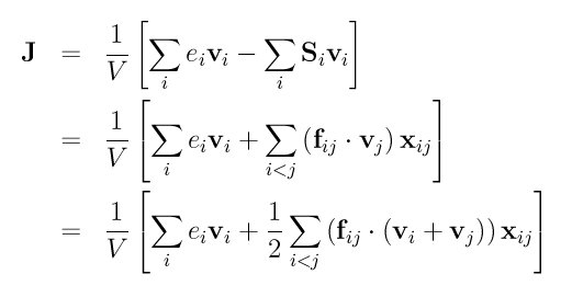
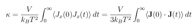
The Green-Kubo formulas relate the ensemble average of the auto-correlation of the heat flux J to the thermal conductivity kappa:
Ei in the first term of the equation for J is the per-atom energy (potential and kinetic). This is calculated by the computes ke-ID and pe-ID. Si in the second term of the equation for J is the per-atom stress tensor calculated by the compute stress-ID. The tensor multiplies Vi as a 3x3 matrix-vector multiply to yield a vector. Note that as discussed below, the 1/V scaling factor in the equation for J is NOT included in the calculation performed by this compute; you need to add it for a volume appropriate to the atoms included in the calculation.
IMPORTANT NOTE: The compute pe/atom and compute stress/atom commands have options for which terms to include in their calculation (pair, bond, etc). The heat flux calculation will thus include exactly the same terms. Normally you should use compute stress/atom virial so as not to include a kinetic energy term in the heat flux.
This compute calculates 6 quantities and stores them in a 6-component vector. The first 3 components are the x, y, z components of the full heat flux vector, i.e. (Jx, Jy, Jz). The next 3 components are the x, y, z components of just the convective portion of the flux, i.e. the first term in the equation for J above.
The heat flux can be output every so many timesteps (e.g. via the thermo_style custom command). Then as a post-processing operation, an autocorrelation can be performed, its integral estimated, and the Green-Kubo formula above evaluated.
The fix ave/correlate command can calclate the autocorrelation. The trap() function in the variable command can calculate the integral.
An example LAMMPS input script for solid Ar is appended below. The result should be: average conductivity ~0.29 in W/mK.
Output info:
This compute calculates a global vector of length 6 (total heat flux vector, followed by conductive heat flux vector), which can be accessed by indices 1-6. These values can be used by any command that uses global vector values from a compute as input. See this section for an overview of LAMMPS output options.
The vector values calculated by this compute are "extensive", meaning they scale with the number of atoms in the simulation. They can be divided by the appropriate volume to get a flux, which would then be an "intensive" value, meaning independent of the number of atoms in the simulation. Note that if the compute is "all", then the appropriate volume to divide by is the simulation box volume. However, if a sub-group is used, it should be the volume containing those atoms.
The vector values will be in energy*velocity units. Once divided by a volume the units will be that of flux, namely energy/area/time units
Restrictions: none
Related commands:
fix thermal/conductivity, fix ave/correlate, variable
Default: none
# Sample LAMMPS input script for thermal conductivity of solid Ar
units       real
variable    T equal 70
variable    V equal vol
variable    dt equal 4.0
variable    p equal 200     # correlation length
variable    s equal 10      # sample interval
variable    d equal $p*$s   # dump interval
# convert from LAMMPS real units to SI
variable    kB equal 1.3806504e-23    # [J/K] Boltzmann
variable    kCal2J equal 4186.0/6.02214e23
variable    A2m equal 1.0e-10
variable    fs2s equal 1.0e-15
variable    convert equal ${kCal2J}*${kCal2J}/${fs2s}/${A2m}
# setup problem
dimension    3
boundary     p p p
lattice      fcc 5.376 orient x 1 0 0 orient y 0 1 0 orient z 0 0 1
region       box block 0 4 0 4 0 4
create_box   1 box
create_atoms 1 box
mass	     1 39.948
pair_style   lj/cut 13.0
pair_coeff   * * 0.2381 3.405
timestep     ${dt}
thermo	     $d
# equilibration and thermalization
velocity     all create $T 102486 mom yes rot yes dist gaussian
fix          NVT all nvt temp $T $T 10 drag 0.2
run          8000
# thermal conductivity calculation, switch to NVE if desired
#unfix       NVT
#fix         NVE all nve
reset_timestep 0
compute      myKE all ke/atom
compute      myPE all pe/atom
compute      myStress all stress/atom virial
compute      flux all heat/flux myKE myPE myStress
variable     Jx equal c_flux[1]/vol
variable     Jy equal c_flux[2]/vol
variable     Jz equal c_flux[3]/vol
fix          JJ all ave/correlate $s $p $d &
             c_flux[1] c_flux[2] c_flux[3] type auto file J0Jt.dat ave running
variable     scale equal ${convert}/${kB}/$T/$T/$V*$s*${dt}
variable     k11 equal trap(f_JJ[3])*${scale}
variable     k22 equal trap(f_JJ[4])*${scale}
variable     k33 equal trap(f_JJ[5])*${scale}
thermo_style custom step temp v_Jx v_Jy v_Jz v_k11 v_k22 v_k33
run          100000
variable     k equal (v_k11+v_k22+v_k33)/3.0
variable     ndens equal count(all)/vol
print        "average conductivity: $k[W/mK] @ $T K, ${ndens} /A^3"